DICOM Image Visualization: ggplot2, Clinical Windows, Shiny, and 3D Volumes

Overview

dicomtk provides a complete medical image visualization pipeline built on native C++17 pixel extraction (read_dicom_pixels()), VOI LUT window/level presets (dicom_window()), composable ggplot2 rendering (plot_dicom() / ggdicom()), an interactive Shiny viewer (dicom_viewer()), and 3D volumetric rendering (render_volume()).

library(dicomtk)
library(ggplot2)
#> Warning: package 'ggplot2' was built under R version 4.5.3

dcm_file <- system.file("extdata", "example.dcm", package = "dicomtk")

Extracting Pixel Data & Applying Clinical Window Presets

read_dicom_pixels() decodes 8-bit, 16-bit, or 32-bit monochrome and RGB pixel streams (including RLE-compressed frames) and applies Modality LUT rescaling (RescaleSlope and RescaleIntercept):

px <- read_dicom_pixels(dcm_file)
dim(px)
#> [1] 512 512

# Apply clinical window presets ("auto", "brain", "stroke", "subdural",
# "lung", "mediastinum", "abdomen", "liver", "bone", "angio")
win_brain <- dicom_window(px, preset = "brain")
range(win_brain)
#> [1] 0 1

Composable ggplot2 Rendering (plot_dicom() & ggdicom())

plot_dicom(dcm_file, window = "auto", palette = "gray", title = "Radiological Grayscale")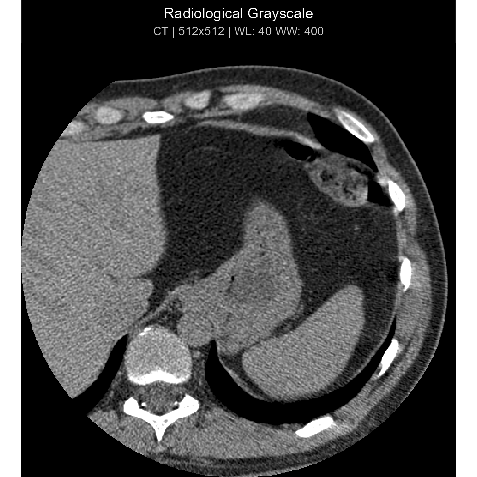

# Add custom ggplot2 annotations on top of ggdicom()
ggdicom(dcm_file, palette = "inferno", annotate = FALSE) +
  labs(title = "Inferno Colormap with Custom ggplot2 Layer")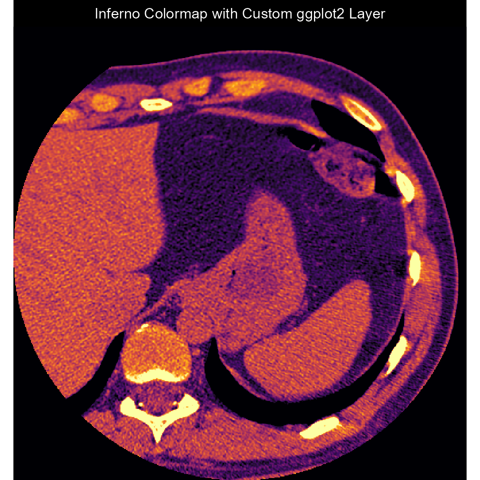

3D Volumetric Multi-Planar Reconstruction (MPR) & Maximum Intensity Projection (MIP)

series <- read_dicom_series(c(dcm_file, dcm_file, dcm_file))
series
#> ℹ DICOM Series: 512 x 512 x 3 slices (3 files)

# 3-Plane Orthogonal MPR
render_volume(series, method = "mpr")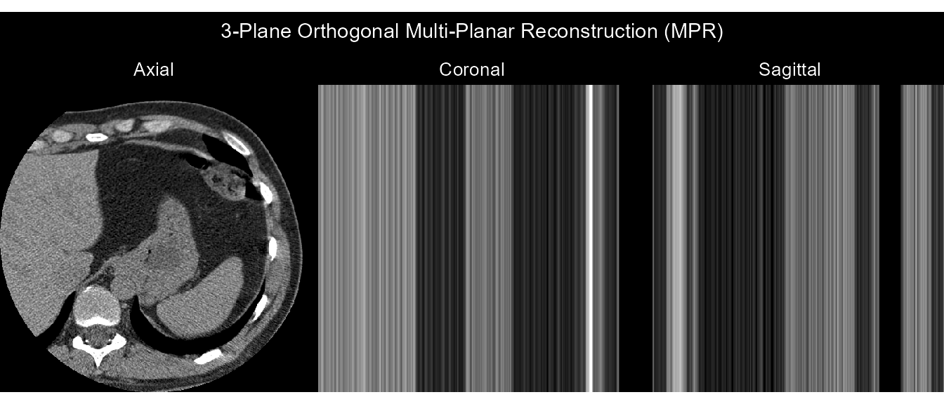

# 3-Plane Maximum Intensity Projection (MIP)
render_volume(series, method = "mip", palette = "viridis")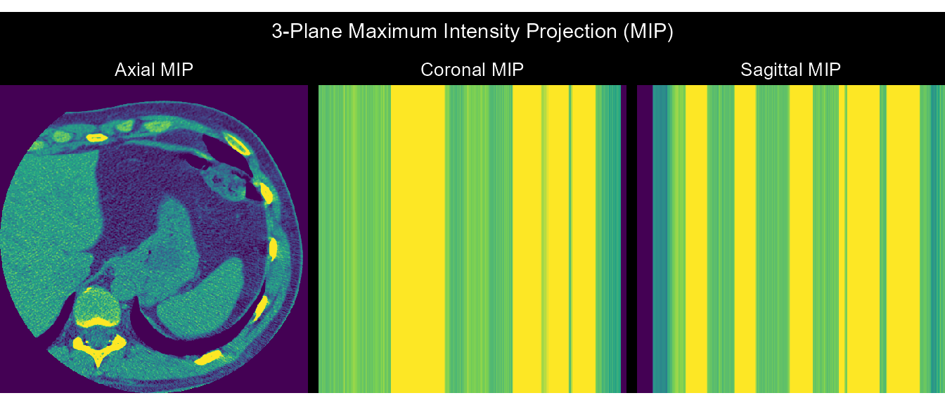

Interactive Shiny Viewer

In an interactive R session, call dicom_viewer() to launch a full multi-slice DICOM workstation in your browser or IDE viewer pane:

if (interactive()) {
  dicom_viewer(dcm_file)
}